Contents
f2py: calling fortran subroutines from python
f2py is an increadibly useful little utility that comes included with numpy. It converts subroutines (and modules) written in Fortran into Python modules, which can then be imported as usual. Why would you want to do that? Well, as covered in a pervious note, Fortran is much better suited for many Monte Carlo applications, while Python is much better for analysing our data. So, why not combine the power of both?
My main interest in this was when building
the onsager library for Python,
which calculates the virial coefficients using Monte Carlo
integration. This would be increadibly slow in Python, as
for higher order coefficients it is not possible to
vectorize the calculation. Instead, the heavy lifting is
done in a Fortran subroutine, while we can use Python to
fit functions or visualize the results, for example. Here,
I will illustrate the basics of using f2py with a simple
example, namely generating random numbers from a
distribution.
Generating random numbers from a polynomial distribution
Feel free to skips this section if you are only interested in using f2py, and not on the specific application.
Lets assume we want to sample random numbers between 0 and 1 from a distribution function which is given by an nth-order polynomial. It takes the form:
where ai are constants that control the
shape of the distribution.
We want to pick nin random values from this
distribution for a given set of ai values. We
will write a subroutine that takes nin and an array of
size n+1 containing the ai values as inputs,
and outputs nin values of x. We will use the
so-called rejection
sampling method to generate the numbers, where x and y
values are chosen. If y < f(x), then we keep x, otherwise
we reject it.
Prerequisites
From the Python side, just Numpy is required in order
to use f2py, though for this example we also need
matplotlib in order to plot the results. From the Fortran
side, a compiler of some sort is required: I use
gfortran.
Writing the Fortran subroutine
We write a Fortran subroutine poly_dist.f90, which looks like this:
 SUBROUTINE sample(var_input, nin, n,  var_output)

  USE funcs                           !use the module funcs which contains random_num and poly_func

  IMPLICIT NONE

  INTEGER :: n                        !the order of the polynomial + 1
  INTEGER :: nin                      !number of random numbers to return
  REAL(8), DIMENSION(n) :: var_input  !coefficients a_i for the polynomial
  REAL(8) :: var_output(nin)          !the random numbers that will be returned

  REAL(8) :: x, y, y_max              !local variables
  INTEGER :: i                        !local variable

  !f2py intent(in) :: var_input, nin
  !f2py intent(hide), depend(var_input) :: n = shape(var_input, 0)
  !f2py intent(out):: var_output

  !seed random number generator
  CALL RANDOM_SEED()

  !set the maximum y value (when x = 1)
  y_max = poly_func(1.0d0, n, var_input)

  !loop from 1 to nin
  DO i = 1,nin

101  x = random_num(         !generate a random number between 0 and   1   for x
     y = y_max*random_num(   !generate a random number between 0 and y_max for y

     !test if y is less than the value of the polynomial
     IF (y .LT. poly_func(x, n, var_input)) THEN
        !if yes, then keep the number and store it as the i-th value to output
        var_output(i) = x
     ELSE
        !if not, then generate new x and y
        GOTO 101
     END IF

  END DO

 END SUBROUTINE sample
Note that there are three lines of code, highlighted in green, which begin with !f2py. These lines will be used by f2py to define the input, output and "hidden" variables:
- !f2py intent(in) :: var_input, nin
- the varibales var_input and nin are required as
inputs when the subroutine is called from
Python.
- !f2py intent(hide), depend(var_input) :: n = shape(var_input, 0)
- the varibale n is not required as an input when
the subroutine is called from Python. Instead, its
value is taken implicitly as the size of the first
dimension of the variable var_input.
- !f2py intent(out) :: var_output
- the varibale var_output is not required as an
input when the subroutine is called from
Python. Instead, when the subrputine is called,
var_output is returned as though a function is
called. If there is more than one variable defined
as output, then are returned as a Tuple in
Python.
This program also uses two functions declared in a separate file, functions.f90, which are stored in a module funcs. These do not have to interface with Python, and are written as normal in Fortran. Note that for the random numbers we're using the inbuilt random number generator. Usually we would NEVER use this (I typically use the GSL generator), but for simplicity we'll use it here.
MODULE funcs

 CONTAINS
  FUNCTION random_num()
    ! function to generate random numbers

    REAL(8) :: random_num

    CALL RANDOM_NUMBER(random_num)

    RETURN
  END FUNCTION random_num


  FUNCTION poly_func(x, n, coeffs)
    ! polynomial function of order n-1 and woth coefficients coeffs

    IMPLICIT NONE

    REAL(8) :: poly_func
    INTEGER :: n
    REAL(8) :: x
    REAL(8) :: coeffs(n)
    REAL(8) :: num, dem
    INTEGER :: i

    num = 0.0d0
    dem = 0.0d0

    DO i = 1,n
       num = num + coeffs(i)*x**(i-1)
       dem = dem + coeffs(i)/dble(i)
    END DO

    poly_func = num/dem
    RETURN

  END FUNCTION poly_func

END MODULE funcs
Compiling the Fortran subroutine
First, we need to compile any additional files, in our case functions.f90
gfortran -c functions.f90
Then we can compile poly_dist.f90 using f2py
python3.5 -m numpy.f2py -c -m poly_dist functions.f90 poly_dist.f90
Here we have specified python3.5, although any
version can be used. The first -m flag tells python to run
the module numpy.f2py as a script. The second -m flag
tells f2py what the name of the module will be, in our
case poly_dist. The -c flag tells f2py that we are
compiling an object file, rather than an
executable.
Using the module in Python
Now we can import the module, along with any others we will need.
		#import the numpy and matplotlib.pyplot
		import numpy as np
		import matplotlib.pyplot as plt
		#import our module
		import poly_dist
Before using our Fortran subroutine, we will first write a Python function to calculate the same polynomial that we will sample from.
		#define a function to calculate the polynomial for a given set of coefficients
		def func(x, coeffs):
		    num = 0.0
		    dem = 0.0
		    for i in range(len(coeffs)):
		        num += coeffs[i]*x**i
		        dem += coeffs[i]/(i+1)
		    return num/dem
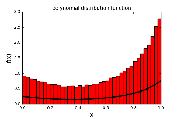
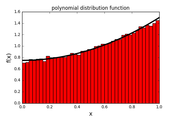
And now we can generate our samples. As a test we will go for an 11th order and a 2nd order polynomial.
		#set the coefficients for an 11th order polynomial
		coeffs1 = [1.0,-2.0,2.0,1.0-1.0,-1.0,-1.0,0.7,1.4,-1.0,0.5,0.5]
		y1 = poly_dist.sample(coeffs1, 100000)

		#set the coefficients for a 2nd order polynomial
		coeffs2 = [1.0,0.0,1.0]
		y2 = poly_dist.sample(coeffs2, 100000)
And finally we can plot the outcome, first for the 11th order, and then the 2nd order polynomials.
		#plot a histogram of the output for the 11th order polynomial
		plt.hist(y1,bins = 40, normed=True, color="red")

		#calculate and plot the actual function
		x_in = np.linspace(0.0,1.0,100)
		y_in1 = func(x_in, coeffs1)
		plt.plot(x_in,y_in1, linewidth=3, c="black")

		#set the title and axis labels
		plt.title("polynomial distribution function")
		plt.xlabel("x")
		plt.ylabel("f(x)")

		#show the plot
		plt.show()

		#plot a histogram of the output for the 11th order polynomial
		plt.hist(y2,bins = 40, normed=True, color="red")

		#calculate and plot the actual function
		x_in = np.linspace(0.0,1.0,100)
		y_in2 = func(x_in, coeffs2)
		plt.plot(x_in,y_in2, linewidth=3, c="black")

		#set the title and axis labels
		plt.title("polynomial distribution function")
		plt.xlabel("x")
		plt.ylabel("f(x)")

		#show the plot
		plt.show()
